PRIDE Archive Project Tagger
A model to automatically assign project tags
PRIDE Archive Project Tagger
Jose A. Dianes
6 April 2015
Introduction and Goals
The PRIDE Archive uses a system of tags to classify datasets. So far these tags are manually assigned by curators. So far the PRIDE teach considers the following tags:
- Biological
- Biomedical
- Cardiovascular
- Chromosome-centric Human Proteome Project (C-HPP)
- Human Proteome Project
- Metaproteomics
- PRIME-XS Project
- Technical
In the present analysis, by trying to build a model that predict tags, we want to find out what are behind those tags. Is it information such as a project species or tissue relevant to identify a project as biomedical? Is it that information actually hidden in the dataset textual description?
Getting and cleaning the data
Let's start by getting the latest prideR version form GitHub, together with
some other packages we will use to build our model.
library(devtools)
install_github("PRIDE-R/prideR")
library(prideR)
require(ggplot2)
theme_set(theme_linedraw())
require(tm)
library(caTools)
library(randomForest)
library(pander)
Now we get all the projects available in the archive.
archive.df <- as.data.frame(search.list.ProjectSummary("",0,20000))Kepp only those with a project tag assigned.
archive.df <- subset(archive.df, project.tags!="Not available")The tags distribution
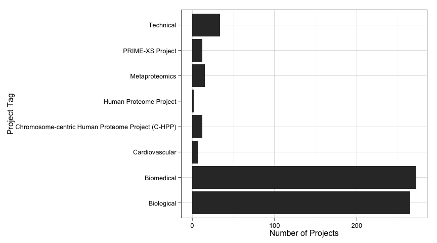
Now we have 619 tagged projects in the dataset. Let's have a quick look at how these tags are distributed.
ggplot(data=archive.df, aes(x=as.factor(archive.df$project.tags))) +
    geom_bar() +
    coord_flip( ) +
    ylab("Number of Projects") +
    xlab("Project Tag")
As we see, our data project tag distribution is very skewed. This will make difficult to build good models, specially now that we have very few projects.
Using meta-data
Let's start by trying to predict projects tags based on meta-data only. That is, by using information such as the species, tissues, and so on.
Preparing meta-data
Right now we have all the metadata associated to PRIDE datasets in text format.
In order to use it to build a model we better convert it to categorica data.
However, most of them have too many differnet values for R machine libraries to
make use of them as predictors. For that reason we need to aggregate those low
frequency values into a unique Other factor level.
species.counts <- table(archive.df$species)
low.freq.species <- as.factor(names(which(species.counts<3)))
archive.df[archive.df$species %in% low.freq.species,]$species <- "Other"
archive.df$species <- as.factor(archive.df$species)

tissues.counts <- table(archive.df$tissues)
low.freq.tissues <- as.factor(names(which(tissues.counts<3)))
archive.df[archive.df$tissues %in% low.freq.tissues,]$tissues <- "Other"
archive.df$tissues <- as.factor(archive.df$tissues)

ptm.counts <- table(archive.df$ptm.names)
low.freq.ptm <- as.factor(names(which(ptm.counts<3)))
archive.df[archive.df$ptm.names %in% low.freq.ptm,]$ptm.names <- "Other"
archive.df$ptm.names <- as.factor(archive.df$ptm.names)

instrument.counts <- table(archive.df$instrument.names)
low.freq.instrument <- as.factor(names(which(instrument.counts<3)))
archive.df[archive.df$instrument.names %in% low.freq.instrument,]$instrument.names <- "Other"
archive.df$instrument.names <- as.factor(archive.df$instrument.names)

archive.df$project.tags <- as.factor(archive.df$project.tags)
archive.df$submissionType <- as.factor(archive.df$submissionType)
Exploring metadata
Let's explore a bit how each piece of metadata is distributed accross each project tag. This might give us some insight into useful predictos if we find any species, tissue, etc., more present in a particular tag than others.
For that we will build a linear model and check the statistical importance of each predictor.
meta_log_model <- glm(
    project.tags ~ species + tissues + ptm.names + instrument.names + num.assays + submissionType,
    data=archive.df,
    family=binomial)
## Warning: glm.fit: fitted probabilities numerically 0 or 1 occurred
meta_log_model_summary <- summary(meta_log_model)
relevant_meta <- names(which(meta_log_model_summary$coefficients[,4]<0.05))
And we see that the following predictors are statistically significan when predicting tags assuming a linear relationship:
| Predictor |
|---|
| speciesHomo sapiens (Human) |
| speciesMus musculus (Mouse) |
| speciesRattus norvegicus (Rat) |
| speciesSus scrofa domesticus (domestic pig) |
| submissionTypePRIDE |
We cannot conclude much due to two factors. First, our relationship is surely not linear. And second, our dataset is too small to model better relationships. But at least it seems to be some relationship between species, and submission type, and the project tag.
A meta-data only model
Let's try now a Random Forest model using just metadata predictors. We know our dependent variable is very skewed, so don't expect too much accuracy. We decide for this type of model due to its success with non-linear problems.
First of all, prepare a train/test split so we can check accuracy. We also have the problem of having too few data in general. Hopefully our models will get better while PRIDE datasets get more numerous.
set.seed(123)
spl <- sample.split(archive.df, .85)

evalTrain <- archive.df[spl==T,]
evalTest <- archive.df[spl==F,]
And now train the model.
set.seed(123)
rfModelMeta <- randomForest(
    project.tags ~ species + tissues + ptm.names + instrument.names + submissionType,
    data = evalTrain)
# Calculate accuracy on the test set
rfPredMeta <- predict(rfModelMeta, newdata=evalTest)
t <- table(evalTest$project.tags, rfPredMeta)
meta_accuracy <- (t[1,1] + t[2,2] + t[3,3] + t[4,4] + t[5,5] + t[6,6] + t[7,7] + t[8,8]) / nrow(evalTest)
We have a prediction accuracy of 0.7232143 on the test data. We can also see how the model struggles to predict on classes with very few cases and does better with large classes.
| Biological | Biomedical | Cardiovascular | Chromosome-centric Human Proteome Project (C-HPP) | Human Proteome Project | Metaproteomics | PRIME-XS Project | Technical | |
|---|---|---|---|---|---|---|---|---|
| Biological | 38 | 8 | 0 | 0 | 0 | 1 | 0 | 1 |
| Biomedical | 8 | 41 | 0 | 0 | 0 | 0 | 0 | 0 |
| Cardiovascular | 0 | 1 | 0 | 0 | 0 | 0 | 0 | 0 |
| Chromosome-centric Human Proteome Project (C-HPP) | 0 | 0 | 0 | 1 | 0 | 0 | 0 | 0 |
| Human Proteome Project | 0 | 0 | 0 | 0 | 0 | 0 | 0 | 0 |
| Metaproteomics | 2 | 3 | 0 | 0 | 0 | 0 | 0 | 0 |
| PRIME-XS Project | 0 | 3 | 0 | 0 | 0 | 0 | 0 | 0 |
| Technical | 2 | 2 | 0 | 0 | 0 | 0 | 0 | 1 |
Using text fields
Surely PRIDE curators use textual description about datasets in order to assign a tag to them. Let's try to incorporate that information into our models in order to predict a dataset tag.
Preparing the corpus
We have two textual fields, project.title and project.description. Let's
prepare a corpus with both of them. In both cases we will reduce them to
lowercase, remove punctuation and stopwords, and apply stemming.
library(tm)
evalTrain$AllText <- do.call(paste, evalTrain[,c("project.title","project.description")])
evalTest$AllText <- do.call(paste, evalTest[,c("project.title","project.description")])

corpusAll <- Corpus(VectorSource(c(evalTrain$AllText, evalTest$AllText)))
corpusAll <- tm_map(corpusAll, tolower)
corpusAll <- tm_map(corpusAll, PlainTextDocument)
corpusAll <- tm_map(corpusAll, removePunctuation)
corpusAll <- tm_map(corpusAll, removeWords, stopwords("english"))
corpusAll <- tm_map(corpusAll, stripWhitespace)
corpusAll <- tm_map(corpusAll, stemDocument)
We will also keep just those terms appearing in at least 3 percent of the projects.
# Generate term matrix
dtmAll <- DocumentTermMatrix(corpusAll)
sparseAll <- removeSparseTerms(dtmAll, 0.99)
allWords <- data.frame(as.matrix(sparseAll))

colnames(allWords) <- make.names(colnames(allWords))
Word clouds
Another useful thing we could do in order to better understand our data is to visualise what words appear more often for a given tag. Doing this visually allows us to grasp the information quickly.
We can use the same approach as before to get the data ready.
corpusCloud <- Corpus(VectorSource(c(evalTrain$AllText, evalTest$AllText)))
corpusCloud <- tm_map(corpusCloud, tolower)
corpusCloud <- tm_map(corpusCloud, PlainTextDocument)
corpusCloud <- tm_map(corpusCloud, removePunctuation)
corpusCloud <- tm_map(corpusCloud, removeWords, stopwords("english"))
corpusCloud <- tm_map(corpusCloud, stripWhitespace)
dtmCloud <- DocumentTermMatrix(corpusCloud)
allCloud <- data.frame(as.matrix(dtmCloud))
Biological word cloud
allCloudBiological <- allCloud[archive.df$project.tag=="Biological",]
wordcloud(colnames(allCloudBiological), colSums(allCloudBiological), scale=c(2,0.25))
Biomedical word cloud
allCloudBiomedical <- allCloud[archive.df$project.tag=="Biomedical",]
wordcloud(colnames(allCloudBiomedical), colSums(allCloudBiomedical), scale=c(2,0.25))
Cardiovascular word cloud
allCloudCardiovascular <- allCloud[archive.df$project.tag=="Cardiovascular",]
wordcloud(colnames(allCloudCardiovascular), colSums(allCloudCardiovascular), scale=c(2,0.25))
C-HPP word cloud
allCloudCHPP <- allCloud[archive.df$project.tag=="Chromosome-centric Human Proteome Project (C-HPP)",]
wordcloud(colnames(allCloudCHPP), colSums(allCloudCHPP), scale=c(2,0.25))
Metaproteomics word cloud
allCloudMetaproteomics <- allCloud[archive.df$project.tag=="Metaproteomics",]
wordcloud(colnames(allCloudMetaproteomics), colSums(allCloudMetaproteomics), scale=c(2,0.25))
PRIME-XS Project word cloud
allCloudPrimeXs <- allCloud[archive.df$project.tag=="PRIME-XS Project",]
wordcloud(colnames(allCloudPrimeXs), colSums(allCloudPrimeXs), scale=c(2,0.25))
Technical word cloud
allCloudTechnical <- allCloud[archive.df$project.tag=="Technical",]
wordcloud(colnames(allCloudTechnical), colSums(allCloudTechnical), scale=c(2,0.25))
Some thoughts about word clouds
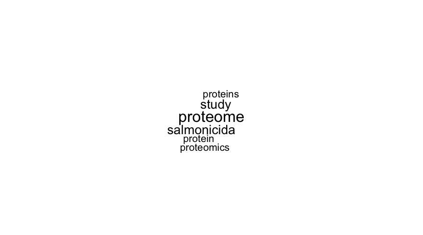
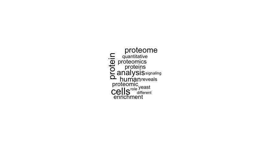
One obvious conclusion that emerges from these charts is that some tags are clearly underrepresented. This will make our models not very efficient. However we can count on this situation to change in the future while more and more projects are submitted to PRIDE Archive.
We can also see that some words rank top in most project tags, and are probably not very useful as predictors. Specially we refer to the family of terms related to proteomics, proteins, etc. We hope these terms will be filtered out in our model selection process in the next section.
Selecting significative terms
We have ended up with 214 possible predictors. But we can do better than this. We are going to train a linear model using them and our dependent variable as outcome. Then we will get those variables that are statistically significative and incorporate them to the main dataset that we will use with our final model.
# Find most significative terms
allWordsTrain2 <- head(allWords, nrow(evalTrain))
allWordsTrain2$Popular <- evalTrain$project.tag
logModelAllWords <- glm(Popular~., data=allWordsTrain2, family=binomial)
all_three_star_terms <- names(which(summary(logModelAllWords)$coefficients[,4]<0.001))
all_two_star_terms <- names(which(summary(logModelAllWords)$coefficients[,4]<0.01))
all_one_star_terms <- names(which(summary(logModelAllWords)$coefficients[,4]<0.05))

# Leave just those terms that are different between popular and unpopular articles
allWords <- subset(allWords,
                   select=names(allWords) %in% all_one_star_terms)

# Split again
allWordsTrain <- head(allWords, nrow(evalTrain))
allWordsTest <- tail(allWords, nrow(evalTest))

# Add to dataframes
evalTrain <- cbind(evalTrain, allWordsTrain)
evalTest <- cbind(evalTest, allWordsTest)

# Remove all text variable since we don't need it
evalTrain$AllText <- NULL
evalTest$AllText <- NULL
We ended up with just 35 predictors that will be incorporated into our model. These are the terms together with their mean frequencies by project tag (remember they are stemmed):
allWords$project.tag <- archive.df$project.tag
panderOptions('round', 2)
panderOptions('keep.trailing.zeros', TRUE)
pander(t(aggregate(.~project.tag, data=allWords, mean)), round=4, style = "rmarkdown", split.table = Inf)| project.tag | Biological | Biomedical | Cardiovascular | Chromosome-centric Human Proteome Project (C-HPP) | Human Proteome Project | Metaproteomics | PRIME-XS Project | Technical |
| aim | 0.01132075 | 0.01838235 | 0.14285714 | 0.00000000 | 0.00000000 | 0.00000000 | 0.08333333 | 0.02941176 |
| analysi | 0.19245283 | 0.20220588 | 0.42857143 | 0.16666667 | 0.50000000 | 0.13333333 | 0.08333333 | 0.20588235 |
| biolog | 0.026415094 | 0.007352941 | 0.000000000 | 0.000000000 | 0.000000000 | 0.000000000 | 0.083333333 | 0.000000000 |
| biomark | 0.01886792 | 0.02205882 | 0.00000000 | 0.08333333 | 0.00000000 | 0.00000000 | 0.00000000 | 0.02941176 |
| brain | 0.01132075 | 0.01838235 | 0.00000000 | 0.00000000 | 0.00000000 | 0.00000000 | 0.00000000 | 0.00000000 |
| combin | 0.02264151 | 0.02941176 | 0.00000000 | 0.00000000 | 0.00000000 | 0.00000000 | 0.00000000 | 0.02941176 |
| comparison | 0.003773585 | 0.011029412 | 0.000000000 | 0.000000000 | 0.000000000 | 0.000000000 | 0.166666667 | 0.029411765 |
| comprehens | 0.03018868 | 0.03308824 | 0.14285714 | 0.00000000 | 0.00000000 | 0.00000000 | 0.00000000 | 0.02941176 |
| control | 0.01886792 | 0.01838235 | 0.00000000 | 0.00000000 | 0.00000000 | 0.00000000 | 0.00000000 | 0.00000000 |
| crucial | 0.01132075 | 0.01838235 | 0.00000000 | 0.00000000 | 0.00000000 | 0.00000000 | 0.00000000 | 0.00000000 |
| dataset | 0.02264151 | 0.02573529 | 0.00000000 | 0.08333333 | 0.00000000 | 0.13333333 | 0.00000000 | 0.02941176 |
| determin | 0.018867925 | 0.007352941 | 0.000000000 | 0.000000000 | 0.000000000 | 0.066666667 | 0.000000000 | 0.029411765 |
| develop | 0.05283019 | 0.03308824 | 0.00000000 | 0.08333333 | 0.00000000 | 0.00000000 | 0.00000000 | 0.02941176 |
| differ | 0.03018868 | 0.04044118 | 0.14285714 | 0.00000000 | 0.00000000 | 0.00000000 | 0.00000000 | 0.11764706 |
| digest | 0.011320755 | 0.007352941 | 0.142857143 | 0.000000000 | 0.000000000 | 0.000000000 | 0.250000000 | 0.058823529 |
| enzym | 0.01509434 | 0.01838235 | 0.00000000 | 0.08333333 | 0.00000000 | 0.00000000 | 0.00000000 | 0.00000000 |
| fluid | 0.02641509 | 0.02573529 | 0.00000000 | 0.08333333 | 0.00000000 | 0.00000000 | 0.00000000 | 0.00000000 |
| human | 0.24905660 | 0.18750000 | 0.14285714 | 0.00000000 | 0.50000000 | 0.06666667 | 0.08333333 | 0.17647059 |
| identifi | 0.04528302 | 0.04044118 | 0.14285714 | 0.25000000 | 0.00000000 | 0.00000000 | 0.08333333 | 0.02941176 |
| impact | 0.01509434 | 0.01102941 | 0.00000000 | 0.08333333 | 0.00000000 | 0.06666667 | 0.00000000 | 0.00000000 |
| investig | 0.02641509 | 0.03308824 | 0.00000000 | 0.00000000 | 0.00000000 | 0.00000000 | 0.08333333 | 0.05882353 |
| itraq | 0.011320755 | 0.007352941 | 0.000000000 | 0.000000000 | 0.000000000 | 0.000000000 | 0.083333333 | 0.029411765 |
| larg | 0.01886792 | 0.01102941 | 0.00000000 | 0.00000000 | 0.50000000 | 0.00000000 | 0.00000000 | 0.00000000 |
| major | 0.011320755 | 0.007352941 | 0.000000000 | 0.083333333 | 0.000000000 | 0.000000000 | 0.083333333 | 0.029411765 |
| mass | 0.08301887 | 0.05147059 | 0.00000000 | 0.00000000 | 0.00000000 | 0.00000000 | 0.00000000 | 0.05882353 |
| modif | 0.026415094 | 0.007352941 | 0.000000000 | 0.000000000 | 0.000000000 | 0.000000000 | 0.000000000 | 0.029411765 |
| pathway | 0.02264151 | 0.01470588 | 0.00000000 | 0.00000000 | 0.00000000 | 0.00000000 | 0.00000000 | 0.00000000 |
| plasma | 0.03018868 | 0.04044118 | 0.00000000 | 0.00000000 | 0.00000000 | 0.00000000 | 0.00000000 | 0.05882353 |
| present | 0.02264151 | 0.02205882 | 0.00000000 | 0.16666667 | 0.00000000 | 0.00000000 | 0.00000000 | 0.00000000 |
| proteogenom | 0.01886792 | 0.01102941 | 0.00000000 | 0.00000000 | 0.00000000 | 0.13333333 | 0.00000000 | 0.00000000 |
| spectrometri | 0.05283019 | 0.02573529 | 0.00000000 | 0.00000000 | 0.00000000 | 0.00000000 | 0.00000000 | 0.02941176 |
| stimul | 0.01509434 | 0.01470588 | 0.00000000 | 0.00000000 | 0.00000000 | 0.00000000 | 0.00000000 | 0.02941176 |
| strategi | 0.02641509 | 0.01838235 | 0.00000000 | 0.00000000 | 0.00000000 | 0.00000000 | 0.00000000 | 0.00000000 |
| system | 0.04905660 | 0.04411765 | 0.14285714 | 0.00000000 | 0.00000000 | 0.00000000 | 0.00000000 | 0.00000000 |
| time | 0.00754717 | 0.02205882 | 0.00000000 | 0.00000000 | 0.00000000 | 0.00000000 | 0.00000000 | 0.00000000 |
A meta-data and text model
So let's train now a model using our meta-data predictors together with those selected in the previous process using textual data.
set.seed(123)
rfModelMetaText <- randomForest(
    project.tags ~ . - accession - publication.date - project.title - project.description,
    data = evalTrain)
# Calculate accuracy on the test set
rfPredMetaText <- predict(rfModelMetaText, newdata=evalTest)
t <- table(evalTest$project.tags, rfPredMetaText)
meta_text_accuracy <- (t[1,1] + t[2,2] + t[3,3] + t[4,4] + t[5,5] + t[6,6] + t[7,7] + t[8,8]) / nrow(evalTest)
We obtain an accuracy of 0.75. The improvement is actually
in better predicting the biological and technical classes a bit.
| Biological | Biomedical | Cardiovascular | Chromosome-centric Human Proteome Project (C-HPP) | Human Proteome Project | Metaproteomics | PRIME-XS Project | Technical | |
|---|---|---|---|---|---|---|---|---|
| Biological | 40 | 8 | 0 | 0 | 0 | 0 | 0 | 0 |
| Biomedical | 8 | 41 | 0 | 0 | 0 | 0 | 0 | 0 |
| Cardiovascular | 0 | 1 | 0 | 0 | 0 | 0 | 0 | 0 |
| Chromosome-centric Human Proteome Project (C-HPP) | 0 | 0 | 0 | 1 | 0 | 0 | 0 | 0 |
| Human Proteome Project | 0 | 0 | 0 | 0 | 0 | 0 | 0 | 0 |
| Metaproteomics | 2 | 3 | 0 | 0 | 0 | 0 | 0 | 0 |
| PRIME-XS Project | 1 | 2 | 0 | 0 | 0 | 0 | 0 | 0 |
| Technical | 2 | 1 | 0 | 0 | 0 | 0 | 0 | 2 |
Conclusions
We have seen our two main problems:
- Our data is very unbalanced. There are many more
biologicalandbiomedicaldata than anything else.
- The previous one becomes more of a problem due to the reduced size of our
training data.
Hopefully both problems will become less and less important with time, while PRIDE gets more submissions.
We have also seen that incorporating textual data to meta-data makes our model more accurate. Not by a lot, but more accurate after all.
In terms of our original questions, we don't have enough confidence neither to predict tags nor to profile each tag in terms of its associated meta-data or textual description (although we have a starting list of candidate terms). However we have seen that there is a relationship, specially when we have enough cases for a given tag to train a model. Additionally we have seen that both things, meta-data and textual description contribute to predict a dataset tag more accuratelly.
Future works
Our simple train/split might be making our model overfit the data. A good approach would be to use cross validation. However, by using random forests we attenuate this problem.
We also need to try different models and do additional exploratory analysis. By doing so we will come with additional insight into the nature of our data. This will help to select variables and even to use other techniques such as ensemble or cluster-then-predict.